A new paper thoroughly examines the empirical performance of leading stock-return predictors. Most predictive variables perform poorly. One variable stands out as a consistent predictor, though: End-of-the-year consumption growth, a variable Stig V. Møller and I introduced in 2015. It feels a little like winning the “world cup in return prediction”.
Stock return predictability is a fascinating topic. Investors would like to know if indicators exist that contain information about the outlook for stocks. Academics also find it interesting, for empirical and theoretical reasons. It is an active research area.
A new paper by Goyal, Welch & Zafirov (link) thoroughly compares the predictive performance of leading predictors. Goyal, Welch & Zafirov evaluate almost 50 variables. These include the short-term interest rate, the term spread, the dividend yield, and many other indicators that academics and practitioners routinely use to judge the outlook for stocks.
The main conclusion of Goyal, Welch & Zafirov is somewhat depressing: “Most variables have already lost their empirical support” and “Overall, the predictive performance remains disappointing.” Most of the variables people look at do not contain a lot of information about future stock returns.
But – and here comes the reason I write this analysis – they also write that “As already hinted, not all variables performed poorly. The empirical analysis suggests some good candidates.”
In particular, Goyal, Welch & Zafirov write (and in the next two lines I directly copy their conclusion):
“The best and most consistent variable was:
Fourth-Quarter Growth Rate in Personal Consumption Expenditures”
The fourth-quarter growth rate in consumption was introduced by Stig V. Møller and myself in 2015 (link). Goyal, Welch & Zafirov have now conducted a very comprehensive evaluation of all the leading predictors out there. They conclude that our variables is “the best and most consistent”.
To understand what happens in the Goyal, Welch & Zafirov paper, and to explain why consumption growth at the end of the year predicts stock returns, let me proceed in several steps. Let me first explain how academics usually evaluate whether indicators contain information about future stock returns. Let me then introduce our variable, i.e. end-of-the-year consumption growth. The paper by Goyal, Welch & Zafirov (2021) builds on the insights of a famous paper Goyal & Welch wrote in 2008 (link). I explain that paper and their new 2021 paper. Finally, I explain why end-of-the-year consumption growth is “the best stock return predictor out there”.
Measuring the predictability of stock returns
Predicting stock returns means finding a today-observable variable that tells us something about future stock returns. Given the obvious importance of this topic for practitioners and academics, many, as in really many, variables have been suggested in the academic literature and by practitioners. In this section, I will illustrate how academics measure return predictability. I will use a famous predictive variable: The short-term interest rate. I will subsequently compare the predictive performance of the short-term interest rate to the predictive performance of end-of-the-year consumption growth.
Campbell introduced in 1987 the short-term interest rate as a stock return predictor (link). The underlying idea is that higher interest rates today hurt future stock returns. This could be because inflation has increased, pushing up the short nominal interest rates. Early papers (e.g., Fama 1981, link) argued that inflation is bad for economic activity and firms’ future output, and hence bad for future stock returns.
Today, we perhaps think more in terms of monetary policy and its effect on firms and stock prices. The central bank hikes the short interest rate when economic conditions are good and lowers it when economic activity suffers. If monetary policy tightening succeeds in taming future economic activity, higher short-term rates today should lower future economic activity and consequently the prospects of firms. This hurts stock returns. In short, changes in the short interest rate today might affect (predict) future stock returns negatively.
I illustrate things here using calendar year (January 1 through December 31) returns from the US stock market. Returns are the returns on the value-weighted stock index including all NYSE, Amex, and Nasdaq stocks, taken from the Center for Research in Security Prices (CRSP). As Goyal and Welch (2008) look at stock returns over and above the short-term risk-free return, i.e. the equity premium, I do the same here. The risk-free return also comes from the CRSP database. The period is 1948-2020.
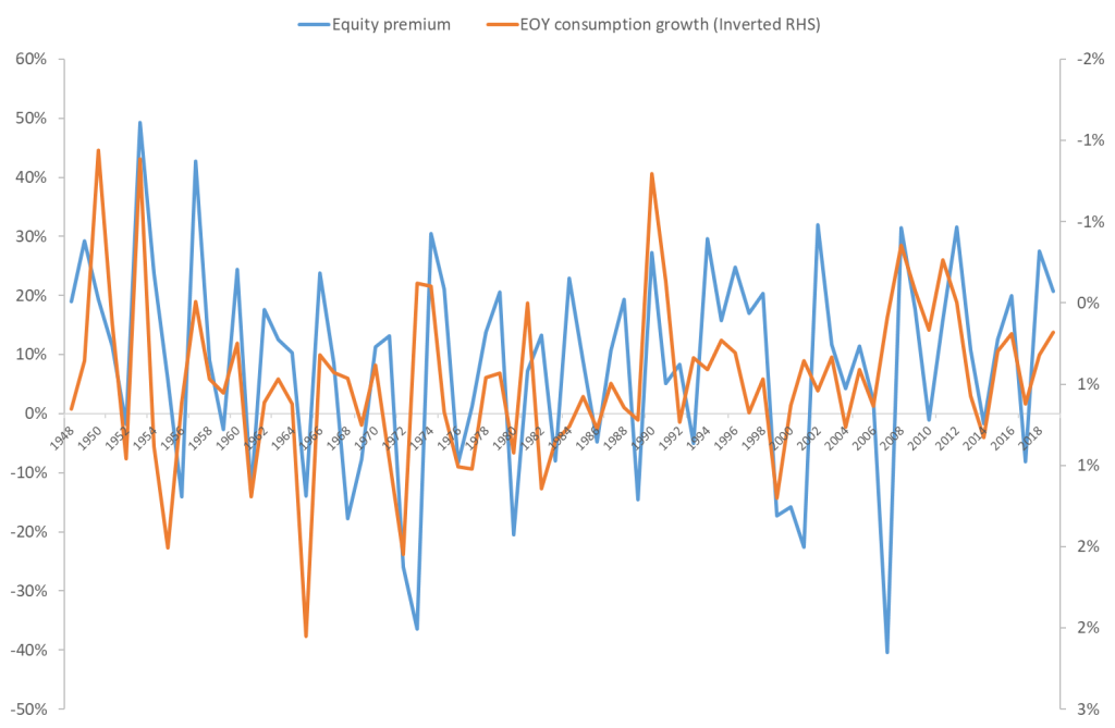
I plot the annual equity premium in Figure 1. The equity premium is volatile. It might be 30% one year, only to be followed by a 0% equity premium next year. It is challenging to find a variable that predicts these large swings in the stock market.
In Figure 1, I also include the short-term interest rate. I use the 3-month Treasury Bill rate at the beginning of each year, i.e. in January. The short-term interest rate relates to the right-hand-side y-axis in Figure 1. I have also inverted the right-hand-side Y-axis to make it easier to see the negative relation between the short-term interest rate and the future equity premium.
Figure 1 asks if there is a relation between the short-term interest rate in the beginning of the year and the equity premium realized over the following year. Basically, if interest rates are low in January, will the return on the stock market over and above the risk-free rate be high going forward?
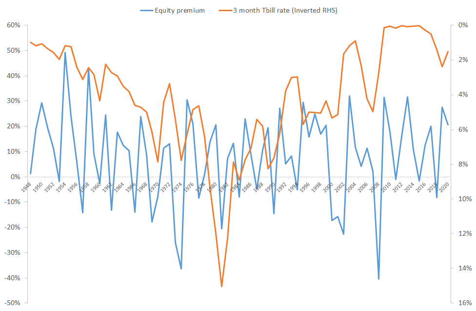
There is no super-strong relation between the two series, but if ones stares closely at Figure 1, one should see a weak relation. There seems to be a tendency that high interest rates in the beginning of the year are followed by a low equity premium during the year, and vice versa. For instance, the interest rate was hiked significantly in 1970, 1974, and 1981. Correspondingly, the equity premium was very low these years: -8% in 1970, -36% in 1974, and – 20% in 1981.
To measure whether there is a statistically significant relation between the short-term interest rate in the beginning of the year and the subsequent equity premium, academics run regressions. I find the following result (I suppress the estimate of the regression constant, as this is not important here):
Excess return = constant – 1.4∙Treasury Bill, t(Tbill) = -2.14 R2 = 6.1%
The estimated regression coefficient is ‘-1.4’. This means that when the short-term interest rate in the beginning of the year is one percentage point higher than it usually is, the subsequent annual equity premium is 1.4% percentage points lower than it would otherwise be. The interest rate predicts future returns with a negative sign. A higher interest rate today means a lower equity premium going forward.
The t-statistic is -2.14. As you remember from your statistics class, this means that the hypothesis that the regression coefficient is equal to zero is accepted with a very low probability only. Or, more directly, the hypothesis that there is no relationship between the short-term interest rate in the beginning of the year and the subsequent equity premium is rejected. Typically, we test at a 5%-level, and the critical value is -1.96. We find here a t-statistic of -2.14, i.e. a smaller coefficient than -1.96. This means that the estimated relation is statistically significant. However, at the same time, the t-statistic is just below -1.96, i.e. the coefficient is just marginally significant.
Finally, the R2 of 6.1% means that variation in the T-bill rate has captured 6.1% of the variation in the annual equity premium.
All in all, there is some, but only some, evidence that hikes in the short-term interest rate lower the future equity premium.
End-of-the-year consumption growth
In 2015, Stig and I introduced growth in aggregate consumption at the end-of-the-year as a stock return predictor (link). We hypothesized that the relation between economic growth and expected returns is stronger at infrequent points in time. We argued:
“When economic fluctuations at the end of the year are relatively more important for business cycle fluctuations (Wen, 2002) and when investors take current economic performance into account when forming expectations about future returns (Campbell and Cochrane, 1999), which they seem to do to a significant extent at the end of the year (Ritter and Chopra, 1989), i.e., investors are lazy (Jagannathan and Wang, 2007) possibly because of information and transaction costs (Abel, Eberly, and Panageas, 2007,2013), expected returns are relatively more affected by end-of-the-year economic activity.”
We thoroughly tested, and verified, that end-of-the-year consumption growth strongly predicts future stock returns. In Figure 2, I show the equity premium (the same equity premium as in Figure 1) and lagged end-of-the-year consumption growth, updated with data until today (in our published 2015 paper, the last observation was 2010). Consumption growth refers to the right-hand-side axis in the figure, and that axis is inverted. We measure end-of-the-year consumption growth as the change in real per capita consumption of nondurables and services from the third quarter to the forth (and last) quarter of the year. These quarterly data are available from 1948. We ask: if consumption growth is high at the end of the year, does it predict the equity premium over the next year?
If you compare Figure 2 with Figure 1, you see that there is a relatively strong relation between the annual equity premium and consumption growth at the end of the previous year. The lines simply line up. End-of-the-year consumption growth predicts the equity premium next year. And it does so considerably better than the short-term interest rate.
This is borne out by the regression results:
Excess return = constant – 15.6∙End-year consumption growth, t(TB) = -4.13 R2 = 19.6%
These results imply that there is a very strong statistical relation between consumption growth at the end of the year and the equity premium over the following year. The t-statistic is -4.13. In these types of regressions, this is (numerically) a very high t-statistic (trust me). It means that we strongly reject the hypothesis that there is no relation between consumption growth at the end of the year and the equity premium next year. The R2 is almost 20%. This means that end-of-the-year consumption growth explains almost three times more of the variation in the equity premium than does the short interest rate. This is impressive. Finally, the sign to the estimated coefficient is negative. This means that when consumption growth at the end of the year is particularly high, the equity premium has a tendency to be low next year. We provide in our paper a framework for thinking about this negative effect. We show that these results are consistent with a habit-formation story, i.e. when current consumption is high, people feel good and are happy to take on more risk in their investments (their risk aversion is low). This pushes up current stock prices and, in the end, lowers expected returns.
In our paper, we show that consumption growth at other times of the year do not predict returns. Only consumption growth at the end of the year predicts returns.
Because these results are and were so amazingly strong, but also intriguing, the referees and the editor made us work hard to rule out all kinds of suspicions. In our paper, we document the results of a painstakingly long list of robustness tests. We (i) run the regressions in alternative ways, (ii) we investigate real and nominal economic growth, (iii) we look at other stock portfolios than the aggregate market, and we look at bond portfolios, (iv) we investigate a lot of the statistical issues that arise when running these types of regressions, (v) we look at other macreconomic variables related to consumption, such as GDP and industrial production, (vi) we investigate monthly industrial production, and we find that December growth in industrial production predicts returns, strengthening our hypothesis that it really is economic growth the end of the year that is special, (vii) we look at consumption series available today (i.e. revised series) and series available to investors in real time, (viii) we do subsample analyses, (ix) we do out-of-sample analyses, and (x) we do a lot of other things. In all these many, many tests, end-of-the-year consumption growth always comes out as a very strong stock return predictor. Finally, and perhaps most importantly, in a follow-up paper we published in 2018 (link), we show that this is not only a US phenomenon. In fact, it is global phenomena. Around the globe, i.e. in international data, there is a clear tendency that stock returns are low following high growth in consumption at the end of the previous year.
Goyal & Welch (2008)
Goyal & Welch (2008) made a landmark, if controversial, contribution to the return predictability literature (link). Their argument was that, OK, you might run regressions such as those I have presented above, but investors will not benefit in real time. Basically, Goyal & Welch (2008) asked, does it help the investor who manages real money to know that stock returns have historically have had a bad year following hikes in the short-term interest rate?
The argument of Goyal & Welch (2008) can be illustrated as follows. Above, I showed that over the full 1948-2020 sample, the relation between the short-term interest rate at the beginning of the year and the subsequently realized equity premium is ‘-1.4’. This relationship – the ‘-1.4’ – is estimated using all data available today, i.e. it is the average relation between the two variables over the full 1948-2020 period.
An investor making an investment in, say, 1970 will not know what the relationship is over the 1948-2020 period. In 1970, the investor will know/can estimate the relation between 1948 and 1970. The investor, of course, does not have perfect foresight.
Running the same regression as the first one above, but for the 1948-1970 period, the estimated relationship is ‘-5.20’. This is a very different estimate than the one we found for the full 1948-2020 period (the ‘-1.4’). For the 1948-1970 period, we find that the equity premium drops by 5% when interest rates are hiked by one percent. Over the full 1948-2020 sample, we find the effect to be -1.4%. It is still a negative relation, but a much smaller one. There is estimation risk. And there is quite a lot of it.
Goyal & Welch (2008) then said: Let us do an exercise. Let us ask what the expected equity premium for 1971 would be if we base that expectation on our knowledge of the relation between the equity premium and the short-term interest rate up until 1970. In other words, what would an investor in 1970 have expected the equity premium to be in 1971? This means using the period 1948-1970 to forecast the equity premium for 1971. Then we do the same for 1972, 1973, etc. We call such forecasts “out-of-sample” forecasts, as opposed to the forecast we get if we use all the information for the 1948-2020 period (called “in-sample forecasts”).
Goyal & Welch (2008) said: Let us compare these out-of-sample forecasts to the simplest forecasts we can imagine: that the equity premium in 1971 will be what it has always been, i.e. its historical average.
The result of this exercise was remarkable. Basically, Goyal & Welch (2008) found, the estimate of the expected equity premium for 1971, based on our knowledge of the relation between the short-term interest rate and the equity premium up until 1970, was no better than simply saying that we expect the equity premium to be what it has been historically.
But it became even worse. In this analysis, I have used the short-term interest rate to illustrate. Goyal & Welch (2008) examined a host of variables that researchers have argued predict returns, such as the dividend yield, the earnings yield, the slope of the term structure, and many others. Around 20 variables in total. Goyal & Welch found that none – none – of them consistently predicted the equity premium more precisely than the historical average of the equity premium. This was of course an embarrassment for the return-predictability literature.
To understand the importance of the Goyal & Welch (2008) result, remember that the finding of time-varying expected returns, and thus return predictability, is often viewed as one of, if not the, most important insight in finance during the past several decades. In his famous “New facts in finance” 1999 survey article (link), Hoover Institution Senior Fellow John Cochrane mentions that until the mid-1980s, people believed that returns were unpredictable. Today, “we know that returns are predictable”. And here come Goyal & Welch, basically saying: “OK, returns might be predictable in a statistical regression, but you cannot use this insight in the real world we are living in. Instead of using fancy tools and regressions, for real-world investors the best guess of the future equity premium is its historical average.” This was obviously provocative. But it was also an important insight. The Goyal & Welch (2008) article has subsequently been cited in more than 3000 academic articles.
Goyal, Welch and Zafirov (2021)
Following the Goyal & Welch (2008) article, researchers have kept on investigating whether expected returns vary over time, and what economic variables characterize such variation. In this recent return-predictability literature, people typically make sure to show that the variable they suggest predicts returns also out-of-sample. This, that researchers today acknowledge that a variable needs to show out-of-sample robustness (in addition to in-sample robustness), is not least due to the influence of the Goyal & Welch (2008) article.
A couple of weeks ago, Goyal & Welch, this time together with Ph.D. student Zafirov, updated their 2008 results. In their original 2008 paper, they use data up until 2005. In their new paper (link), they update with recent data to see if their results still hold. In addition, they include a large number of predictive variables developed since their 2008 paper. They include 29 new variables from 26 academic articles, all published in top-academic journals since 2008. One of the new variables they include is our end-of-the-year consumption growth.
In their investigation, Goyal, Welch & Zafirov follow the same procedure as the one they used in their original 2008 paper, examining both in-sample and out-of-sample performance of the different variables.
Their conclusion is that “Overall, the predictive performance remains disappointing”.
Regarding the new variables they investigate in data spanning until 2020, they conclude: “Most variables have already lost their empirical support”.
But Goyal, Welch & Zafirov also conclude, and this is of course what Stig and I find most interesting:
“As already hinted, not all variables performed poorly. The empirical analysis suggests some good candidates. The best and most consistent variable was:
Fourth-Quarter Growth Rate in Personal Consumption Expenditures (gpce) was introduced in Møller and Rangvid (2015). High personal consumption growth rates this year predict poor stock-market returns next year.
Empirically, since the 1970s, gpce has only made one modest misstep in its predictive ability (which was missing the Great Recession bear market). Otherwise, gpce has been a steady performer.”
Goyal, Welch & Zafirov use the same outcome variable (the equity premium), the same techniques, same procedures, everything done by them, and so on – i.e. they do a very clean and comprehensive horserace between variables that have been argued to predict stock returns – and conclude that our variable is the most consistent stock-return predictor.
Illustrating the consistent predictive performance of end-of-the-year consumption growth
The point of Goyal and Welch is that there is estimation uncertainty and coefficient estimates are unstable. The relation that existed between two variables over the 1948-1970 period is often very different from the relation that exists over the 1948-2020 period, as illustrated above with the relation between the equity premium and the short interest rate.
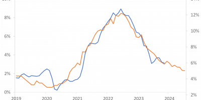
The point here is that the relation between end-of-the-year consumption growth and the future equity premium is stable over time. Figure 3 illustrates. The figure shows the time-series variation in the coefficient estimates of the relation between the future equity premium and the short interest rate, respectively end-of-the-year consumption growth. I show the percentage annual deviation from the mean of the coefficient estimate. In other words, I estimate the relation between the short interest rate in the beginning of the year and the subsequent equity premium using data for the 1948-1970 period. I remember the coefficient estimate. Then I estimate it for the 1948-1971 period. Then for the 1948-1972 period. And so on. I thus generate a time-series of coefficient estimates. This is called recursive estimation. I take the mean of that time series to find the average coefficient estimate. In Figure 4, I plot the percentage difference between the coefficient estimate in a given year and the mean of the time-series of coefficient estimates. So, for instance, in 1970, the estimate of the relation between the equity premium and the interest rate for the 1948-1970 period was almost 150% larger than the mean of all coefficient estimates. I do the same exercise for the relation between the future equity premium and end-of-the-year consumption growth.
The main point of Figure 3 is that there is a lot of time-series variation in the regression coefficient to the short interest rate. The blue line goes from +200% to -50%. On the other hand, as should be clear from the figure, there is a stable and robust relation between end-of-the-year consumption growth and next year’s equity premium. Goyal, Welch & Zafirov document that no other variable generates an equally robust relation over post-World War II period, where quarterly consumption growth is available. Simply, end-of-the-year consumption growth is the best equity-premium predictor out there, over this sample period at least.
There is a case to be made that end-of-the-year consumption growth should be the new benchmark against which we measure predictive variables. To make it easy for other researchers to implement tests using end-of-the-year consumption growth, I have uploaded the data to my webpage (link).
Conclusion
The finding that expected returns are not constant but vary over time in systematic ways with predictive variables is one of the great discoveries of the past four decades of research in finance. It means that returns are predictable and that asset prices do not follow random walks. The implications for academics, investors, and financial markets almost cannot be overstated.
Goyal & Welch (2008) published a thought-provocative paper arguing that we might be able to demonstrate historical equity-premium predictability, but there is so much variation in the estimated relationship between predictive variables and the future equity premium that this predictability is not relevant for real-world investors. This was a thought-provoking insight.
Now, Goyal, Welch & Zafirov (2021) have produced a new paper where they update and expand upon their initial 2008 paper. They include new predictive variables introduced since 2008. One of the variables they examine is end-of-the-year consumption growth that Stig V. Moeller and I introduced in 2015. We hypothesized and showed empirically that consumption growth at the end of the year is a strong predictor of the future equity premium.
Overall, Goyal, Welch & Zafirov (2021) argue that the evidence in favor of predictability generally “remains unimpressive”.
They also argue, however, and this is the point I would like to emphasize in this analysis, that some variables show strong and robust predictive power. In particular, they find that “the best and most consistent variable” is consumption growth at the end of the year. These are interesting results. Smart people (Goyal, Welch, and Zafirov) have compared a large number of predictive variables. Ours come out on top. It feels like winning the world-cup in return prediction.