Some of the events we have seen during this crisis are so unlikely that we need tricks to calculate their probabilities. This is a journey into the world of very small probabilities and very large numbers. I admit it is somewhat surreal. But it is important as these small-probability events can have long-lasting effects on economic activity.
The defining characteristic of this recession is the speed with which markets and economies started freefalling. From one day to the next, economies were shut down. Economic activity came to a complete sudden stop in some sectors. In different blogposts, I have used words such as “unprecedented”, “completely crazy”, “horrifying”, “tremendous”, etc. to describe what happened.
Using words like these is adequate, I think (I admit I was shocked by what happened), but I have come to a point where I want to be more precise. As economists, we want to put numbers on things. I want to calculate the probability of the events. This turned out to be more complicated than I had first imagined.
The probability of a 121-sigma event
On Monday, April 20, the oil price (West Texas Intermediate) closed at USD -38 for a barrel of oil. I describe this here (link). This was a drop of 306% relative to the closing price the previous trading day. Based on daily data since 1983, the average percentage change in the oil price is 0.03% and the standard deviation 2.5%. I called the event “completely crazy”, which I still believe is a fair description. Now, I want to know “how crazy” it was. What was the probability that it would happen?
The happy-go-lucky Professor of Finance, i.e. me, opens his Excel spreadsheet and enters the command used to find the probability that an event of -306 happens when data are normally distributed with mean 0.03 and standard deviation 2.5.
I press “Enter”. Excel returns “0”. The Professor of Finance thinks this look strange and increases the number of decimal places. Excel just shows “0.000….”. According to Excel, this is a zero-probability event. It could not happen.
But it did happen. I start remembering the statistic classes many years ago, and recall the discussions on low-probability events.
Luckily, I have helpful colleagues. I write CBS Professor of Statistics Søren Feodor Nielsen. He tells me that the probability I am looking for is below the “machine precision”. He also tells me that the probability itself might be extreme, but the logarithm to the probability is probably not. We calculate the log-probability (using a different statistical package than Excel). It is -7495.137, i.e. the likelihood is exp(-7495.137). This is, unfortunately, such a low number that a computer cannot calculate this either.
We then calculate the log base 10 probability. Now we have the result. The probability is 0.799 x 10^(-3255).
This is a zero followed by 3255 zeroes, and then 799. Practically zero, but not exactly zero. The event happened, but it is extremely unlikely. We can call it “completely crazy”, but we can also say that the probability is 0.799 x 10^(-3255).
There is another way to illustrate how unlikely this event was. When the probability is 0.799 x 10^(-3255), we should see this event happen every 1.2516 x 10^(3255) days. I.e., a number with 3255 numbers before the decimal place. I simply do not know what such a number is called (link). This is where it starts getting surreal.
How precise is this? We have calculated it, but Søren tells me we should not put too much faith in its precision. Tail-probabilities in the normal distribution are calculated by numerical approximations, and it is questionable how precise they are when we are that far out in tail. Admittedly, the question is of course also how important it is that it is precise that far out in the tail. The probability is unbelievably small. That is the main thing. Exactly how small is perhaps not that important.
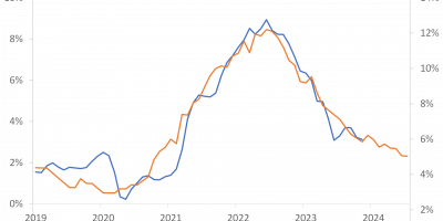
S&P 500
This graph shows daily percentage changes in the S&P 500 throughout the last 50 years.

Data source: Thomson Reuter Datastream via Eikon.
On March 13, the S&P 500 fell 12%. The average daily percentage change in the S&P 500 (calculated up until March 12) is 0.03% and the standard deviation is 1.05%.
The likelihood that we will see a 12% drop in the S&P 500 on a daily basis, given the behavior of the S&P 500 during the last 50 years, is very small, but not so small that it cannot be calculated in Excel. Excel says it is 1.0827 x 10^(-29).
These are daily data. If we assume 250 trading days per year, we should see this event happen every 3.69 x 10^(27) = 3,694,454,429,465,560,000,000,000,000 year. I.e., every 3.694 octillion year.
This is also somewhat surreal.
There are many caveats. We are again so far out in the tail that we should not put too much emphasis on the exact number of decimals and the exact number after all the zeroes. Also, all these calculations are based on the assumption of normally distributed data. Given that we saw a 21% fall in the S&P 500 on Black Monday, October 19, 1987, we have seen two very unlikely crashes within the last three decades. According to these calculations, they should happen much more seldom. We use the normal distribution, but data might follow a different distribution. For most practical purposes, however, it is not necessary to know the exact distribution of these extreme events. The important thing to know is that the likelihood is very small.
Other numbers
In this post (link), I describe how the initial jobless claims soared, confidence indicators fell, GDP dropped, etc. As an example, the likelihood that we should see almost 7 million people filing for jobless claims on March 28, given the complete previous history of jobless weekly claims, is 0.97 x 10^(-841). This is again such a small probability that Excel cannot even calculate it.
Economic effects
There is a broader point to these discussions. Events like those described above might have long-lasting consequences for economic activity.
When events are unlikely, we assign low probability to their occurrence. One hypothesis is that we keep on assigning low probabilities to their occurrence. In this case, future investment decisions of firms and future consumption decisions of households are unaltered by the events we have been going through. It was a temporary shock. It has very low probability. It will not influence how we form expectations going forward.
An alternative hypothesis is that we have become so scared by the event that it will haunt us for years to come. We update our beliefs disproportionally much.
Which of the two scenarios play out is important for the recovery from this recession. Will we start consuming when economies open up or will we hold back because we have become scared?
Kozlowski, Veldkamp and Venkateswaran (2020) have an important paper on this (link). Their main point is that events like those studied above, i.e. events that are very unlikely but have large impacts, will have persistent effects on beliefs. They write that “tail events trigger larger belief revisions” and that “because it will take many more observations of non-tail events to convince someone that the tail event really is unlikely, changes in tail beliefs are particularly persistent”. This is an important insight. If this is how we form expectations, it will slow down the recovery from this recession. Kozlowski et al. also show, however, how government interventions can reduce the effect, but not eliminate it.
Conclusion
These weeks we are seeing infection rates declining in many countries and economies opening up again. These are very good news. Let us hope we can start returning to some kind of normality. It will take time before we are back to where we came from, though. Some things might even have changed for good. One thing is for sure: we will not get back as fast as economies and markets fell in March. What happened was very unlikely. But it did happen.